ESPaDOnS is provided with a data reduction package, called Libre-ESpRIT. Here is the table of content for this page:
Libre-ESpRIT also comes with a script to automatically reduce whatever data has been obtained so far during the night. Plotting tools are presented on the CFHT tools page.
ESpRIT is a self-contained data reduction package developed specifically for reducing echelle spectropolarimetric data . It was developed in 1995 by Donati et al. (1997, MNRAS 291, 658) and implements the principles of optimal extraction as presented by Horne (1986, PASP 98, 609) and further revised by Marsh (1989, PASP 101, 1032). ESpRIT was also generalized to retrieve polarimetric information from echelle spectra with curved orders and tilted slits.
ESpRIT was extensively used in the 1980's to extract spectropolarimetric and spectroscopic data obtained at the 3.9m Anglo-Australian Telescope (ucles spectrograph + sempol polarimeter) and at the 2m Bernard Lyot Telescope (MuSiCoS spectropolarimeter).
Libre-ESpRIT is the new release of ESpRIT , and is the version used with ESPaDOnS at CFHT. In addition to being much more automated than its predecessor, a number of new important features are now available and many critical operations are significantly improved both for reliability and accuracy. As opposed to ESpRIT (which can be distributed to its users), it has been decided by J.-F. Donati that Libre-ESpRIT will not be available outside of CFHT ('Libre' meaning here 'autonomous' or 'independent from others' rather than 'available to others'). The binary files will be operational at CFHT for processing ESPaDOnS data, but observers will not be able to bring those binary files (nor the source code) back home, for any reason, unless explicit written agreement under strict and predefined conditions is obtained before hand from J.-F. Donati.
The data reduction instructions for ESpRIT and Musicos are available at http://webast.ast.obs-mip.fr/magnetisme/pol/esprit.html.
The data reduction instructions for Libre-ESpRIT and ESPaDOnS are available at http://webast.ast.obs-mip.fr/magnetisme/espadons_new/reduction.html.
Data reduction for CCD frames usually includes subtraction of a bias and/or dark frame (a single frame or an average of many frames), and correction for pixel-to-pixel variations in sensitivity (using flat field frames). Bad pixels (dead pixels or hot pixels) can also be masked (ignored by the data reduction software) if a bad pixel map is prepared.
For spectroscopy, one has to find the relationship between a pixel's position on the chip and the wavelength recorded at that pixel. This is done using comparison exposures made with Thorium (Th) lamps (Thorium/Argon, Thorium/Neon, etc.) and/or Fabry-Perot exposures (which use a Fabry-Perot interferometer and the light coming from a flat field lamp). The spectrum is recorded in 2D and has to be collapsed (or extracted) into a 1D spectra.
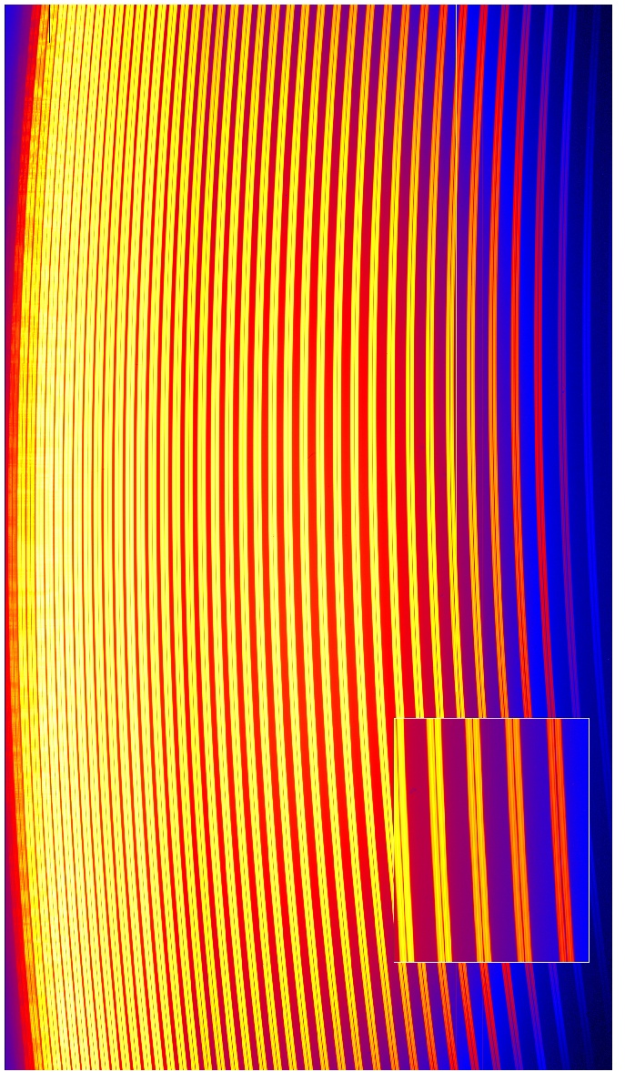
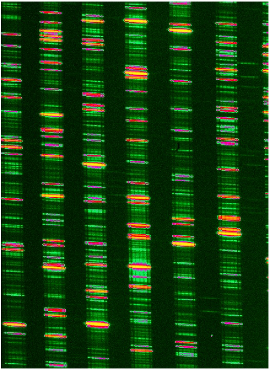
ESPaDOnS records 40 orders, and each one of them is curved [image]. The curvature has to be taken into account (fit) by the software. A zoom of a Thorium lamp exposure shows that the slit is also tilted (no parallel to lines), which is also usually fit [zoom on Th lines].
Libre-ESpRIT will reduce the data obtained with ESPaDOnS in any of the 3 modes.
Libre-ESpRIT proceeds in 2 general steps:
Libre-ESpRIT is a data reduction package for reducing echelle spectropolarimetric data that:
There are a few things that Libre-ESpRIT does not do:
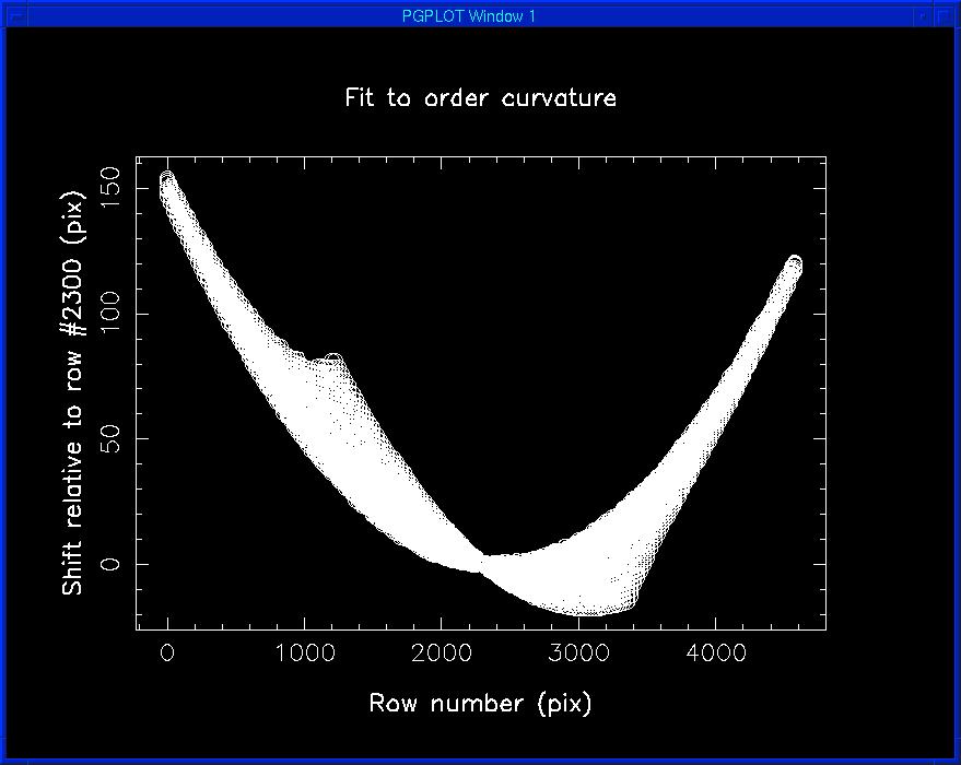
The first step starts with finding all orders present on the CCD and tracking them across their free spectral range (full length of the order). The derived positions are then fitted by a 2-dimensional polynome (with a typical rms accuracy of better than 0.05~px). The graphical result of this operation [graph] shows the estimated and fitted lateral shifts of the 40 orders with respect to their position at mid CCD, plotted as a function of row number (circles depicting measurements and lines representing the fit). The longest orders are the red ones (orders number 22 and above), while the shortest orders are the blue ones (orders 61 and below), the free spectral range of an order being inversely proportional to the order number. Note the difference in scale between both axes.
The direction and shape of the slit formed by the image slicer at spectrograph entry is then evaluated across each order from a comparison frame (either a Th/Ar or a Fabry-Perot frame) and fitted by a low order 2-dimensional polynome depending on both order number and distance from order center (for the slit direction) plus a multi-parametric shift function depending on distance from order center only (for the slit shape, assumed to be identical for all orders).
The previous two pieces of information are then merged together to derive a new curvilinear coordinate system for each order, with one coordinate being the distance from order center and the second one the distance along the order from the slit position at the first pixel of the order. The comparison frame is then extracted within this curvilinear system to obtain a Th/Ar spectrum, with flux as a function of distance along each order.
The frames needed for the routine geometry are:
The program assumes that a single bias frame will be given, but the reduction will work with an average bias frame (except that the readout noise computed will not be right), a single dark, or an average dark frame. The bias subtraction is not a pixel by pixel subtraction (i.e., the reduction does not take the value at a given science pixel and subtract the corresponding value of the bias pixel). The bias frame is divided in 8px by 8px squares, where bad pixels are ignored. The bias values in each 8px by 8px square are averaged, and that grid of values is fit. The fit is subtracted from all other exposures. Therefore, only a single bias frame is required. It is however recommended that 3 biases be taken, so that if one bias does not look right, one of the other 2 can be used (if only 2 biases are taken, it could be unclear which one is the best). It is currently NOT possible to do a pixel-by-pixel subtraction of the bias.
The bias frame is also used to calculate the readout noise. The calculation assumes that only a single frame is given; if an average bias frame is given as input, the readout noise value will be lower. The noise is calculated in 8px by 8px squares. The accuracy of the bias fit should be roughly the value of the readout noise divided by 8. Equivalently, the readout noise will be about 8 times the accuracy of the bias fit.
Each mode requires its own set of calibrations. The reason is related to the choice of fibers in each mode. Three fibers are used, but the pair used in polarimetric mode is different than the pair used in spectroscopic mode star + sky. The spectroscopic mode star only uses only one of the 3 fibers. Therefore, depending on which fiber is used, the light will fall on a different spot on the chip.
If there is not enough flux in the blue, the data reduction will not be able to find the bluest orders. If a flat is saturated in the red, geometry might still work, but the rest of the data reduction will not be possible since the science frames are divided by the flat field. It is therefore crucial that the flats be checked for saturation as soon as they are taken.
The Thorium exposure is only used (geometry) to track the slit. That exposure often has saturated lines in the red. The code tries to fit a Gaussian to each line, and when it fails (if the line is saturated for example), that line is ignored. Therefore, saturated lines in the Thorium exposures are not a problem (saturated lines in science exposures are not a problem either).
In the polarimetric and 'star only' modes, a Fabry-Perot (FP) exposure does a better job of tracking and fitting the shape of the slit than the Thorium exposure. If a FP exposure is not available, one can use the Th/Ar frame instead, but this is not recommended.
The routine creates a file with the geometrical information, and the reduced comparison ThAr spectrum. It is HIGHLY recommended that the output produced be saved, so one can come back to the results of a previous reduction to spot possible problems or discrepancies.
Here is an example of a run, with excepts of the output produced:
Byte swap on FITS files
Flat field :
Name of file to read FITS data from : spec/18oct2004/f1.fits
spec/18oct2004/f1.fits ('test object'       )
Th/Ar :
Name of file to read FITS data from : raw/762865c.fits
raw/762865c.fits ('test object'       )
Fabry-Perot :
Name of file to read FITS data from : raw/762866a.fits
raw/762866a.fits ('test object'       )
Bias :
Name of file to read FITS data from : raw/762864b.fits
raw/762864b.fits ('test object'       )
Name of file to read bad ccd pixel list from : /h/espadons/esprit/src/badpix_eeveng
/h/espadons/esprit/src/badpix_eeveng
Full CCD is [2080:4640]
Input CCD subformat (pix0, npix for each axis) : 8 2040 4 4600
8 2040 4 4600
Is dispersion along CCD columns (y/n) : y
yes
Is wavelength increasing with pixel along orders (y/n) : y
yes
Do you want to invert orders (y/n) n
no
Trimming and transforming data files...
Trimming and transforming data files...
Trimming and transforming data files...
Trimming and transforming data files...
Trimming and transforming data files...
Removing bias...
   Accuracy of 2d bias fit : 0.41 ADU; Readout noise : 3.27 ADU
Centre point of first order (at row #2300) : 41
41.00
Approximate separation between orders : 30
30
Number of first order and order increment towards top of CCD : 22 1
22 1
Maximum number of orders [default = 460] : 40
Extraction length (longest order), midpoint and slope in CCD pix [sug
5900 2300 0] : 7000 2300 -500
7000 2300 -500
Spectral sampling in CCD pix [sug 0.6923] : 0.6923
Counting and locating orders...
   Found 40 orders on CCD
   Rms accuracy of fit to order position: 0.100 pxl
   Order # 22 is centred at column #  31.9 (vertical range: [0 4599]
pxl)
   Order # 23 is centred at column #  62.6 (vertical range: [0 4599]
pxl)
   Order # 24 is centred at column #  93.2 (vertical range: [0 4599]
pxl)
   Order # 25 is centred at column # 124.0 (vertical range: [0 4599]
pxl)
[...]
   Order # 60 is centred at column #1893.1 (vertical range: [1219 3381]
pxl)
   Order # 61 is centred at column #1977.8 (vertical range: [1237 3363]
pxl)
Measuring order curvature...
   Order # 61 limited from pix 1625 to 3363
   Rms accuracy of 2d fit to order location : 0.029 pix
Building coordinate system...
Looking for columns with more than 5.00% of maximum flux...
   Order # 22 : columns -13.2 to 14.0
   Order # 23 : columns -13.2 to 13.6
   Order # 24 : columns -13.2 to 13.6
   Order # 25 : columns -13.2 to 13.6
   Order # 26 : columns -13.2 to 13.6
[...]
   Order # 26 : columns -13.2 to 13.6
[...]
   Order # 60 : columns -14.4 to 14.8
   Order # 61 : columns -13.6 to 14.0
Correcting pixel to pixel sensitivity differences...
Do you want to model slit curvature (y/n) :  y
yes
Measuring slit direction and shape...
   Rms accuracy of 2d fit to slit direction and shape : 0.021 pix
Building coordinate system...
Setting subpixel span...
Name of file to save geometry info to : results/geom.dat
results/geom.dat
Do you want to save the reduced comparison spectrum (y/n) : y
yes
Collapsing frame columns...
   Collapsing order #22
   Collapsing order #23
[...]
   Collapsing order #60
   Collapsing order #61
Name of file to save Stokes profiles to : results/thor.s
results/thor.s
The value for the center point of the first order (at row 2300) can be easily checked by displaying an image of a flat field exposure. One must find the first order with a reasonable amount of light (not the extra order sometimes seen but just very barely). With ds9 and because of definitions of CCD size and data sections, there is a shift of 10px between the position read with the cursor and the number to enter: take the value given by ds9 and subtract 10. If the wrong value is entered, the routine will crash.
The spectral sampling 0.6923 is given in pixels. This is about half a resolution element. One resolution element is about 1.4px, or 2.6 km/s. Therefore, the spectral sampling is about 0.7px, or 1.8 km/s. This value is also the first value in the ThAr spectra produced by geometry.
A good or typical value for the Rms accuracy of fit to order position is 0.02-0.03px. Above 0.1 or 0.2px, an rms value would indicate that there is problem.
A typical value for the Rms accuracy of the 2-dimensional fit to the slit direction and shape is usually 0.02px, but can go up to 0.1px. A value above 0.1px would indicate a problem.
The subpixel span uses the spectral sampling value of 0.6923 pixels. Roughly speaking, the chip gets divided in pixels smaller than the physical pixels (pixels about 0.7px on a side).
During the collapsing of the columns, the fluxes for each wavelength are just added together. There is no optimal extraction done at this stage.
The ThAr spectrum produced by the previous routine geometry is used to find the details of the wavelength to pixel relationship at the center of each order (the dispersion relation); to achieve this, the code starts by searching, fitting and identifying thorium lines iteratively in each order, then fits with a 2-dimensional polynome the position of all lines successfully identified (up to several thousands typically) as a function of both order number and distance along the order. With this scheme, each line effectively participates, not only in the wavelength calibration of a single order, but also in the wavelength calibration of all orders simultaneously, making this process very robust and accurate. The typical rms precision of the derived wavelength calibration at any given pixel is about 150m/s.
The minimum number of lines needed is 40 lines in the red, and 10-20 in the bluest orders. This is usually achieved with the exposure times recommended.
The routine wcal needs:
For each order, there is a rms value given for the preliminary calibration. The rms is first obtained per pixel, then transformed per km/s. A typical value for the rms accuracy is 0.1-0.2 km/s. If something is wrong with an order, the rms value will be around 4-5 km/s (or more). At the end, a mean accuracy for all orders is given. This mean is an average performed after rejecting bad points. A typical value for this mean is less than 0.2 km/s. A value above 0.3-0.4 km/s would indicate a problem.
For each order, there is a max dev value given; a normal value is 0.5 km/s.
For each order, with the mean spectral resolution, there is a lines number given; this is the number of lines in the ThAr exposure used to calculate the resolution.
For each order, a list of lines rejected is given. The dev value for each line is given. The criteria for rejection is a dev value higher than 10.
The Overlap accuracy is based on the lines found on more than one order.
Here is a typical run, with the output produced by the the routine:
Uncalibrated spectrum of comparison lamp : Name of file to read Stokes I
profiles from : results/thor27oct.s
Name of file to read geometry info from : results/geom27oct.dat
Order to be calibrated first : 32
Do you want to use an a priori wavelength calibration table (y/n) : yes
Name of file to read calibration table from :
/h/espadons/esprit/src/calibref.dat
Name of file to read th-ar line wavelengths from :
/h/espadons/esprit/src/thar.arc
Identifying comparison lines in order #22...
   Line @ 1007.9542 nm not found in spectrum
   Feature @ pix 103.34 (~1008.2860 nm) identified as line @ 1008.2879
nm
   Feature @ pix 112.33 (~1008.3782 nm) identified as line @ 1008.3785
nm
   Feature @ pix 164.58 (~1008.9130 nm) identified as line @ 1008.9135
nm
   Feature @ pix 164.58 FINALLY identified as line @ 1008.9135 nm
   Line @ 1009.4265 nm not found in spectrum
   Line @ 1010.2575 nm not found in spectrum
   Feature @ pix 321.40 (~1010.5081 nm) identified as line @ 1010.5077nm
[...]

   Line @ 1047.0054 nm not found in spectrum
   Line @ 1047.8083 nm not found in spectrum
   Preliminary calibration of order #22 : rms acc. 0.233 km/s
       (Order #22 : pix0 = 1007.2233 nm; dlam = 0.0103182 nm/pix; quad =
-3.02481e-07 nm/pix^2)

Identifying comparison lines in order #23...
   Feature @ pix 83.55 (~964.2471 nm) identified as line @ 964.2477 nm
[...]
   Preliminary calibration of order #61 : rms acc. 0.235 km/s
       (Order #61 : pix0 = 363.1122 nm; dlam = 0.00377638 nm/pix; quad =
-1.16072e-07 nm/pix^2)

Rejecting blended lines...
   Order #22 :
      Line @ 1008.9135 nm rejected
      Line @ 1011.1874 nm rejected
   Order #23 :
      Line @ 967.6102 nm rejected
[...]
   Order #61 :
      Line @ 369.1876 nm rejected
      Line @ 369.3995 nm rejected
      Line @ 370.7004 nm rejected
      Line @ 372.2115 nm rejected

Calibrating orders #22 to #61...
   >>> Mean rms accuracy : 0.128 km/s
   Rms accuracy of order #22 calibration : 0.237 km/s (max dev : 0.563km/s)
   Mean spectral resolution in order #22 : 64943 (acc : 1986, #lines :28)
      Line @ 968.2219 pm rejected (dev = 5.877 km/s)
      Line @ 986.5558 pm rejected (dev = -3.301 km/s)
   Rms accuracy of order #23 calibration : 0.178 km/s (max dev : 0.486km/s)
   Mean spectral resolution in order #23 : 67308 (acc : 1267, #lines :59)
      Line @ 931.0444 pm rejected (dev = 4.520 km/s)
      Line @ 931.3800 pm rejected (dev = 5.560 km/s)
[...]
Checking calibration from orders overlap...
   Overlap accuracy between orders #23 and #22 :
   Overlap accuracy between orders #24 and #23 :
   Overlap accuracy between orders #25 and #24 :
   Overlap accuracy between orders #26 and #25 :
   Overlap accuracy between orders #27 and #26 :
       0.124 pix @ 853.0911 nm (respective shifts of  0.064 km/s and -0.257 km/s)
       0.008 pix @ 853.1451 nm (respective shifts of -0.043 km/s and -0.064 km/s)
       0.033 pix @ 853.4680 nm (respective shifts of  0.043 km/s and -0.043 km/s)
       0.033 pix @ 853.4680 nm (respective shifts of  0.043 km/s and -0.043 km/s
[...]
   Overlap accuracy between orders #61 and #60 :
       0.056 pix @ 373.7512 nm (respective shifts of  0.196 km/s and 0.049 km/s)
      -0.038 pix @ 373.7889 nm (respective shifts of -0.196 km/s and -0.098 km/s)
       0.028 pix @ 374.1183 nm (respective shifts of -0.049 km/s and -0.122 km/s)
       0.019 pix @ 374.2923 nm (respective shifts of -0.073 km/s and -0.122 km/s)

Name of file to save Stokes profiles to : results/thor27oct.ws
Name of file to save calibration table from : results/calib27oct.dat
In the following step, optimal extraction of each order is performed, using the curvilinear coordinate system set up with geometry and wcal. The details of the optimal extraction technique can be found in the papers by Horne (1986, PASP 98, 609) and by Marsh (1989, PASP 101, 1032). For polarimetric observations, the optimally extracted spectra from each sub-exposure and each polarization state are then combined together in a specific way to obtain the intensity, polarization and check spectra, along with the error bars associated to each spectrum point (routine polar). The detailed formulas can be found in the paper Donati et al. (1997, MNRAS 291, 58). For data obtained in the spectroscopic object + sky mode, the sky subtraction is performed (routine extract_sky). For all modes, the routine extract can be used. Finally, automatic continuum normalization and wavelength calibration (with the dispersion polynomes derived above) of the resulting spectra are performed, and radial velocity corrections from earth spin and orbit motions are applied to the wavelength scale before storing the final result into a multicolumn ASCII file.
A complete spectrum obtained with ESPaDOnS and reduced with Libre-ESpRIT is worth about 190,000 data points, each point corresponding to a velocity bin of 1.8km/s.
The frames and information needed for the routines are:
The input values for the detector gain and readout noise are used to calculate the noise for each pixel and to calculate error bars. If the values entered are wrong, the error bars will be incorrect.
If the user enters 'no' when asked about the optimal extraction, no optimal extraction will be performed, only an ordinary collapse (add all the pixels along a row).
The rejection threshold is given in sigma, and is mostly used to reject cosmic rays. A low rejection threshold will leave more undesirable pixels, while a high rejection threshold will remove too many pixels (including good ones).
The bias is used to do a 2-dimensional fit of the background, averaged in 8 by 8 pixel boxes. A typical value for the Reduced chisq of 2d background fit is of the order of 1.0; value can sometimes go up to 2 or 3. Higher values (up to 10 for example) might indicate a problem due to scattered light or frost.
When extracting the spectrum, pixels are rejected based on their standard deviation (deviation above 10, the default value). The value val given for each pixel is the value at that pixel.
The Flat field response was computed using a spectrum of the Sun taken with ESPaDOnS. After that correction is made, the spectra of a blue star (hot) will roughly be a negative slope, with a lot of flux in the blue, and less flux in the red, and the spectrum of a red star (cold) will have a positive slope, with more flux in the red than in the blue. The continuum normalization that follows that step will remove the slope to give a flat (horizontal) continuum.
If the user does not use that flat field response, the continuum will look worse than if it used.
Note that for spectra with strong emission lines, the reduction with or without the continuum normalization will look similar.
Also note that for spectra with a lot of emission lines, the reduced data might look better without the continuum normalization. The reason is that typical (or frequent) emission lines found mostly in young stars are considered when doing the continuum normalization, but if a lot of other emission lines are present (other type of star), the continuum normalization will try to consider those lines, and the result might look bad.
At the end, in the SN statistics, the wavelengths given are the wavelengths at the center of each order. The signal-to-noise ratio (SNR) is given in terms of spec pxl, the spectral pixel (spectral resolution element) which defines the spectral resolution and is smaller than a physical CCD pixel. The SNR is also given per CCD pxl, meaning per physical pixel on the chip.
Here is the output of a typical run with extract:
Byte swap on FITS files
Star :
Name of file to read FITS data from : raw/760432o.fits ('test object'   )
Flat field :
Name of file to read FITS data from : spec/26oct2004/f2.fits ('test object'  )
Bias :
Name of file to read FITS data from : raw/760404b.fits ('test object'   )
Name of file to read geometry info from : results/geom27oct.dat
Detector gain (e/ADU) and read-out noise (e) : 1.270 3.260
Optimal extraction of spectrum (y/n) : yes
Rejection threshold [default = 10.0] : 10.0
Name of file to read bad ccd pixel list from :
/h/espadons/esprit/src/badpix_eeveng
Trimming and transforming data files...
Trimming and transforming data files...
Trimming and transforming data files...
Trimming and transforming data files...
Removing bias...
   Accuracy of 2d bias fit : 0.41 ADU; Readout noise : 3.26 ADU
Setting up error bars array...
Building coordinate system...
Computing fractional order position of image pixels...
Looking for columns with more than 1.00% of maximum flux...
   Order # 22 : columns -14.4 to 13.6
   Order # 23 : columns -14.4 to 13.6
[...]
   Order # 56 : columns -14.4 to 15.6
   Order # 57 : columns -13.2 to 14.8
Correcting pixel to pixel sensitivity differences...
Removing background...
   Reduced chisq of 2d background fit : 0.72
Normalising to flat field flux...
Optimal extraction of spectrum...
   Extracting order #22
   Rejecting pixel @ [ 275:4597] (val : -3.034e-04, dev : 84.45 sig)
   Rejecting pixel @ [ 275:4599] (val : -2.895e-04, dev : 74.55 sig)
[...]
   Rejecting pixel @ [ 288:4597] (val : 3.714e-03, dev : 11.15 sig)
   Reduced chisq of optimal extraction fit : 1.349

   Extracting order #23
   Rejecting pixel @ [ 285:4523] (val : -2.347e-04, dev : 47.30 sig)
   Rejecting pixel @ [ 285:4522] (val : -2.007e-04, dev : 44.80 sig)
[...]
Do you have calibration information : yes
Name of file to read calibration table from : results/calib27oct.dat
Correcting wavelength scale from Earth motion...
   Coordinates of object : 15:27:50.96 &  29: 6:31.6
   Time of observations : 2004  9  4 @ UT  7: 8:24 (HA = 4.220 hr)
   Total exposure time : 60.0 s
   Cosine latitude of observatory : 0.941
   Heliocentric velocity of Earth towards star : -17.380 km/s
   Julian date of observation : 2453252.7975
Do you want to divide out spectrum by flat field response : no
Do you want spectrum continuum to be normalised : no
Displaying SN statistics...
   SNR per spec/ccd pxl in order #  57 (398 nm):   I>   15 /   17
   SNR per spec/ccd pxl in order #  56 (404 nm):   I>   32 /   37
[...]
   SNR per spec/ccd pxl in order #  23 (985 nm):   I>  312 /  374
   SNR per spec/ccd pxl in order #  22 (1029 nm):   I>  274 /  328
Name of file to save Stokes profiles to : spec/test.s
The routine produces one plot per order.
The routine extract_sky is used to subtract the sky spectra from the object spectra (in the spectroscopic mode object+sky only).
The result ascii files in spectroscopy modes have the following columns:
The routine polar does the same extraction as in extract, but for 2 or 4 exposures. It also computes polarization.
The routine polar accommodate one important option:
The output consists of one file with 6 columns, as can be seen in the following example:
***Reduced spectrum of '        '
 177362 5
  368.6595 -3.4794e-01  0.0000e+00  0.0000e+00  0.0000e+00  3.5753e-01
  368.6619  8.9022e-01  1.4267e-01  1.4267e-01  9.8503e-02  3.4259e-01
  368.6642 -4.9273e-01  0.0000e+00  0.0000e+00  0.0000e+00  3.1784e-01
[...]
The first line indicates what is the content of the file, along with the object name (blank here). The second line presents the number of lines (or wavelengths) in the file, with the number of columns after the first column. The first column is the wavelength in nm, followed by the intensity (flux), the polarization (one of the Stokes parameters: V, Q, or U), 2 check spectra, and an error bar.
A run with polar resembles a run with extract, except that operations are done on 2 or 4 exposures, not just one. The output of the routine includes strings such as Exposure \#3/4 : to indicate which image is being analyzed. In addition, polarization calculation.
This is the echelle spectra reduction tool 'Libre ESpRIT'
Libre ESpRIT tcsh script:        version 1.06 (2005 Dec 26)
Libre ESpRIT reduction routines: version 2.10
NOTE: Libre ESpRIT is not available for other purposes or at any other
location than CFHT
      If users choose to process ESPaDOnS data with Libre ESpRIT, they
explicitly agree to acknowledge its use and provide appropriate
references in all resulting publications.
      All relevant information about Libre ESpRIT can be found in :
      Donati J-F, Semel M, Carter BD, Rees DE, Cameron AC: 1997, MNRAS 291, 658
      Donati J-F, Catala C, Landstreet JD, et al: 2006, MNRAS (in preparation)

Syntax:  libre_esprit [-scNiplkdrwo] date
arguments: date: local date of the frames to be processed in format ddmmmyy
(eg 17Feb05)
    options:  -s: performs byte swap on fits files
              -c: cancels continuum polarisation automatic removal
              -N: cancels automatic spectrum normalisation
              -i: changes sign of extracted polarisation spectrum
              -p: computes polarisation spectra from sequences only
              -l: starts by cleaning existing log file produced by
                  previous ESpRIT requests
              -k: starts by cleaning existing calibration files produced
                  by previous ESpRIT requests
              -d: starts by cleaning existing reduction lists produced
                  by previous ESpRIT requests
              -r: starts by cleaning existing reduction spectra produced
                  by previous ESpRIT requests
              -w: cancels automatic wavelength correction from telluric lines
              -o: uses badpix file for engineering eev detector
              -g: displays calibration graphs
Segmentation faults
Segmentation faults will occur if the correct directories (results, src)
and essential files do not exist. Check if you have really created the
subdirectories you need.
pgplot error messages
If the path information for pgplot is not there, there will be a message:
PGPLOT /xw: Couldn't find program "pgxwin_server" in the directory named
PGPLOT /xw: in your PGPLOT_DIR environment variable, or in any directory
PGPLOT /xw: listed in your PATH environment variable.
WARNING in ccf2 : 6.723543 outside of [-3.000000 2.000000]
This error is related to a cross-correlation calculation. The high value
(here 6.723543) is the maximum of the cross-correlation, which should be
in the range indicated between the [].