The binary Kuiper Belt Object 1998 WW31 - Chapter 3

Going to Space...

C. Veillet - CFHT
2002 April 13
 
Back to the 1998WW31 story


After the discovery of the binarity and the use of whatever ground based observation available, it was time to go to space and use the high resolution imaging capabilities of the Hubble Space Telescope to nail down the orbit of the pair. For this new phase, the work has been done through a close collaboration between Joel Parker (SWRI), Ian Griffin (STScI) and myself.


First Director's Discretionary Time (DDT) allocation (9259)...

 
We obtained DDT  to observe 1998 WW31 with the Wide Field Planetary Camera 2 (WFPC2) instrument once a month for three months.  The first observations were scheduled at the earliest possible date, early July 2001, when the solar elongation angle of 1998 WW31 was larger than the HST solar avoidance angle.

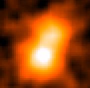
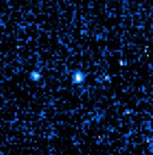
For each of our observations 1998 WW31 was centered on the planetary camera CCD, giving a resolution of 0.046 arc seconds per pixel. With a separation on the sky of ~0.7 arc-seconds the two components were easily resolved. Observations were obtained at three separate epochs: 12 July, 9 August, and 10 September 2001. At each epoch 2 exposures were made through each of the F555W, F675W and F814W filters (comparable to the Johnson system V, R, and I filters).

The animation on the right shows the two components on these three epochs nearly a months apart, with the faint component moving with respect to the bright one kept fixed on the animation. Form month to month, the components are getting closer and closer. On the last one, the separation between them is 0.59 arc-seconds.
 

...while still observing from the ground
 
As soon as 1998 WW31 became visible again in the Summer of 2001, we kept observing the pair with the CFHT 3.6-m telescope using CFH12K, the very same CCD mosaic camera used for the initial discovery of the binary. Thanks to very good seeing, some of the images were nicely showing the pair, even when the components were getting closer. On the left is an image obtained with CFH12K on a night of excellent seeing (0.5") on September 12.5, and on the right an image of the pair as seen by HST on September 9.7. The separation between the two components is only 0.59". These simultaneous observations allowed us to check our estimate of the accuracy of the CFHT measurements against independent and more accurate ones. 

 
With the availability of three HST data points and the series of CFHT measurements more or less at the same epochs, we were able to get an orbit based on what could be considered as a good set of data: old sparse and relatively poor observations (but for those obtained at maximum elongation at the end of 2000 / early 2001) providing a long time span, and high accuracy positions on a short interval of time thanks to HST.

Surprise: No way a circular orbit could fit the data... The path of one component with respect to the other is a highly elongated orbit. The eccentricity is however poorly  constrained by the observations we have, and could be anywhere between 0.5 and ... 0.99!

Why is the eccentricity so important? In fact, the maximum elongation between the two components seem well determined. The semi-major axis (a)  then depends on the eccentricity (e) as the distance at maximum elongation is given by a(1+e). Why is a that important? Because, combined with the period, it will give the mass of the system (see here for more details).


Well... here we are, frustrated again! We had thought the orbit would be more or less determined, and it is not. It is eccentric, but we don't know for sure how eccentric. Assuming e=0.6, we can predict that the pericenter (where the real distance between the pair is minimal) could be reached  in January/February. Obervations around that period would be fantastic to get the eccentricty accurately!

So, back to paper work and a new request for DDT, this time for once a month in late December, January and February.


Second Director's Discretionary Time allocation (9320)
 
The first two observations were obtained on 30 December 2001 and 19 January 2002. An additional set of HST observations made on 13 December 2001, obtained as part of a separate program were graciously made available to us by K. Noll, the PI of that program. 

Oops... Yet another surprise: We missed the pericenter! The eccentricity is higher (~0.8) than we predicted, and the components passed the pericenter earlier than anticipated. 

The plot on the right shows the final orbit (the one published in Nature on Apr. 18, 2002). There is fact one more observation obtained since the paper was finalized. It confirms the current results well within their uncertainty. 


The three positions from (9320) are shown on the animation on the left. You can see how the images look different from the first set. Well, HST didn't change and the weather didn't either (!). What changed is the way the images were processed and smoothed...

On the first of the sequence (December 30), the separation between the components is 0.42 arc-seconds.

The two components are now going away from each other. We really missed the pericenter! Next time is in more than a year and a half. Too bad :(


The results so far...
 
What do we start from?

The data we get by analyzing the images is a set of coordinates of one component with respect to the other on at various epochs. We chose the brightest one as the reference: It is likely to be the bigger one and satisfies our mental image of a small body orbiting a bigger one (like the Earth around the Sun or the Moon around the Earth). In the 1998WW31 pair however, as we shall see later, the two bodies are very similar in size, so our mental image is not going to be close to the reality. 
We also extract from the original images their apparent brightness as seen from Earth or HST at the time of the observations, not only in one, but in three colors, a useful information for the study of their surface.

What do we get?

From the positions, we are able to determine the orbit of one around the other one. The more points we have, or the more precise and accurate the measurements are, or the larger the time span, the better the orbit we get!

Here are a few parameters of the orbital motion:
 
Period (P) ~570 days
Semi-major axis (a) ~22,000 km
Eccentricity (e) ~0.82

As the orbit is far to be circular (unlike the Earth around the Sun or the Moon around the Earth, which are both close to a circular orbit), the distance between the two companions vary by a factor of ten from 4,000 km to 40,000 km.

With an orbit we are able to predict how the pair is going to look like in the future (not too far though because the orbit is not that accurate yet), a few years from now... We can predict that there is going to be a time where we will see the orbit edge on, an opportunity to see one passing in front of the other one and to accurately determine the size of bodies. The current prediction is that it would happen in 50 years from now. It is not even sure that we could see such a pass: With such a long orbital period, the two bodies have to be aligned at the right time...

The last direct information we get, using the period and the semi-major axis, is the total mass of the pair (see here for details). We find that, together, the two components of 1998 WW31 are 1/6000th of the mass of Pluto/Charon, the only pair known in the Kuiper belt before 1998 WW31 was found double.

What do we infer?

From now on, any conclusion is based on at least one assumption, and in some case two or more, while what has been said so far is only a direct consequence of the observations and of the laws of physics as we know them today.

  • Assumption 1 (A1): The two companions have similar surface properties (same global average dust coverage, giving them a same albedo, a quantity that characterizes the amount of light reflected by the surface).
  • Assumption 2 (A2): The two companions have the same density. Basically, they are made of the same material, rock, ice, a mix of the two...
- A1 allows us to translate the difference in brightness into a relative size of the two bodies. 
- A2 allows us to transform a size ratio in a mass ratio

Here is a summary of the results we get, depending on which assumption(s) we use.
 

Assumption made
Information used
Parameter determined
Value(s) found
A1 
Relative brightness
Diameter Ratio
1.2
A1 + A2
Diameter Ratio and Mass
Mass ratio
1.74
A1 + A2 + density = 2 g/cm3
Mass ratio and density
Diameter of each component
~120km, ~100km
"
Diameter and brightness
Albedo
~0.09
A1 + A2 + density = 1.5 g/cm3
Mass ratio and density
Diameter of each component
~130km, ~110km
"
Diameter and brightness
Albedo
~0.07
A1 + A2 + density = 1 g/cm3
Mass ratio and density
Diameter of each component
~150km, ~120km
"
Diameter and brightness
Albedo
~0.05

The size of the components in the 100-150km range, based on reasonable assumptions...

An albedo of 0.04 , a value typical of a cometary nucleus and generally assumed for the KBO's, would give a density slightly smaller than 1 g/cm3, a much lower value than Pluto's density. Though we don't know much on the comet nuclei density, values in the 0.3-1.2 g/cm3 are often mentioned in the literature, which seems to fit our duo!