| SITELLE Home |
| CFHT Home |
| General Information |
| News |
| Instrument Description |
| Fourier Transform Spectroscopy |
| FTS-Primer |
| Publications & SV data |
| Presentations and publications |
| Science Verification data |
| Acknowledgment Text |
| Specifications & Performance |
| Specifications |
| Technical considerations |
| Filters |
| Observing with SITELLE |
| Observations Cookbook |
| Exposure Time Calculator |
| Queued Service Observing * |
| SkyProbe * |
| Data Preprocessing & Calibration |
| ORBS data processing pipeline |
| Standard Stars |
| CFHT MetaData Products |
| Calibration Images Archive |
| ORCS line fitting tool |
| Real Time Image Processing |
| Twilight Flat-Fields Status |
| Focus Sequences Status |
| Calibration Stars Status |
| Spectral Flat Status |
| Instrument Operations |
| Cooling Status* |
| Cryostat Status * |
| External Related Sites |
| Data Archiving at CADC * |
| Contacts |
| Support Astronomers |
| Outreach |
| SITELLE 1st Light |
| * = External Browser Link |
| Imaging Fourier Transform Spectroscopy | ||||||||||||||||||||||||||||||||||||||||||
|
References: books by Vidi Saptari (FTS Instrumentation Engineering), Sumner P. Davis (Fourier Transform Spectrometry), Robert J. Bell (Introductory Fourier Transform Spectroscopy) ; articles by Jean Pierre Maillard (Exp.Astron 2013, 35:527-559)
SITELLE is an imaging Fourier transform spectrometer, or IFTS. An IFTS is a type of integral field unit (IFU) spectroscopy instruments, which give the spectra of all the pixels in their field of view. Other classes of IFU spectrographs use, for instance, long-slit grating spectrometers or Fabry-Perot interferometers. An IFTS combines a 2D imaging detector with a Michelson interferometer. The interferometer scans the optical path difference (OPD) in a step-by-step scanning mode, and the imaging detector records the 2D interferogram of the entire field of view of the instrument at once, for each OPD step. The 3D spectral cube is then recovered after Fourier transform of the 3D interferogram. A schematic view of a Michelson interferometer is shown in Figure 1. Figure: Schematic view of a classical Michelson: as the mirror #2 moves, the observed intensity on the detector varies
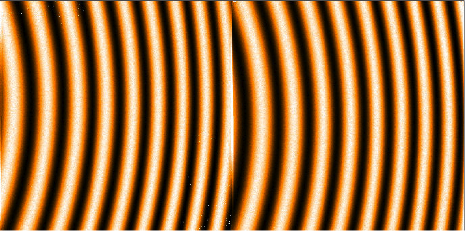
Dual port MichelsonSITELLE uses a dual-port Michelson interferometer: both output beams are recorded onto their own imaging detector. In the classical Michelson interferometer, half of the incident energy is lost as half the light goes back to the source after the second pass in the beamsplitter. The ability to recover both outputs is obtained, for instance, by using corner cube mirrors instead of the flat mirrors, so that the output beams are not superposed with the input beams. Another solution consists of an off-axis design, which is the choice made for SITELLE. The output beam that would normally go back to the source thus becomes accessible, which theoretically doubles the amount of photons the instrument collects with respect to a single port interferometer. Because the sum of the two outputs shall remain constant as a function of OPD, a dual-port FTS also allows to trace changes in flux due to variable observing conditions. Interferograms cubes instead of spectral cubesUnlike a spectrograph that would observe a different wavelength element at each "step", an IFTS observe the whole incident bandpass but at a different OPD element at each step. This is a fundamental difference, which is then found in the product of an observation sequence: SITELLE does not produce two spectral cubes - one for each camera - but their Fourier transforms. As the OPD is scanned by moving one mirror away from the zero path difference (ZPD), fringes appear and "move" on both detectors. The OPD is indeed not constant across the entire field of view because the incident angles of the beams vary from pixel to pixel. In the classical Michelson with perfectly parallel mirrors, the fringes form circles on the detector. Because SITELLE uses an off-axis design, the incident angles are never equal to zero, the detectors do not image the center of the circles, but rather their edges. Figure 2 shows fringes obtained with a monochromatic source on the SITELLE cameras, away from ZPD. Fig 2: 532 nm laser fringe images taken with the SITELLE science cameras (channel 1 at left, channel 2 at right).
What is thus recorded on each detector, at each OPD step, is a 2D image of the sky with fringes. Once that many OPD have been scanned, and after astrometric realignment of all the images to correct for any distortion/drift during the scan, the images are combined into two 3D interferograms. An interferogram is thus obtained for each camera pixel, and it is its Fourier transform that allows the observer to recover the spectrum at that position in the sky. Advantages of the IFTSThe IFTS has several advantages, when compared to other forms of integral field spectrometers. For instance, it is fully flexible in terms of the spectral resolution used to observe, from 1 to that defined by the maximum OPD. The IFTS is in particular known for the following two advantages. First, there is the multiplex or Felgett advantage, according to which the signal-to-noise ratio of an IFTS is significantly better because the entire bandpass is observed at each step, rather than just a spectral element as in a dispersive spectrograph. Then, there is the throughput or Jacquinot advantage, which states that an IFTS can gather significantly more power that a dispersive spectrometer, assuming similar spectral resolution and collecting area. ApodizationThe apodization is related to the fact that the OPD is only scanned over a finite range. To remove the sidelobes that are introduced in the spectra because of the finite OPD range, the interferograms can be multiplied by an apodizing function. A side effect of the apodization is that it lowers the spectral resolution of the spectra. For instance, with a triangular apodization, the width of the lines is increased by about 50%. Whether or not the observers will apodize their interferograms, and what function they will use to do so, will depend on their science goals, and on the strength and number of the lines. The apodization can be performed at any time once the data of been obtained.Spectral resolutionThe resolution of a spectrum produced by an IFTS depends on the maximum OPD scanned, and on the apodization. In the case of the unapodized spectrum, the resolution expressed as a wavenumber is $δσ = 1{/(2L)}$. In the case on the apodized spectrum, using a triangular function, the resolution is lower: $δσ = 1{/L}$. Therefore, the larger the resolution an observer wants to reach, the larger OPD range should be scanned. The choice of the apodization function is also critical.AliasingThe interferogram measured in an IFTS is a sampled version of the theoretical continuous interferogram, Fourier transform of the source spectrum. The sampling of the interferogram introduces an aliasing (i.e. a repeat, or overlap) of the spectrum over a frequency range that is inversely proportional to the OPD sample. In order to observe frequencies from 0 to $σ_{max}$, one should define an OPD sample interval $∆δ ≤ 1{/(2 × σ_{max})} $. | ||||||||||||||||||||||||||||||||||||||||||
| Fundamentals of Fourier transform spectroscopy and theoretical presentation of the IFTS | ||||||||||||||||||||||||||||||||||||||||||
|
At each OPD step, two images of the field of view, with fringes, are saved. For any given pixel (x,y) of each detector, we can write the resulting interferograms I1 and I2, both functions of the OPD ($δ$): $$I_1(x,y,δ) = ∫_{-∞}^{+∞} B(x,y,σ) \[ 1 + \cos(2πσδ)\] dσ$$ and $$I_2(x,y,δ) = ∫_{-∞}^{+∞} B(x,y,σ) \[ 1 - \cos(2πσδ)\] dσ$$ The simple methodConsider the incident electric field: $$ E(x,σ) = E_0(σ) × e^{i(ωt-2πxσ)} $$ After going through the Michelson interferometer, each beam suffers a reflection and a transmission at the beamsplitter (with coefficient $r$ and $t$), and travels along a path that induces a delay $δ$ between both beams. The output amplitude then is: $$ E'(x,σ,δ) = r×t×E_0(σ)×[e^{i(ωt-2πxσ)} + e^{i(ωt-2π(x-δ)σ)}] $$ The corresponding flux is: $$ I'(σ,δ) = |r×t×E_0(σ)|^2 × (1 + \cos(2πδσ)) $$ which can be summed over all wavenumbers: $$ I'(δ) = 2 × ∫_{0}^{∞}|r×t×E_0(σ)|^2 × (1 + \cos(2πδσ)) × dσ $$ From there we infer: $$ I'(0) = 4 × ∫_{0}^{∞}|r×t×E_0(σ)|^2 dσ $$ and hence: $$ I'(δ)- {I'(0)}/2 = 2 × |r×t|^2 × ∫_{0}^{∞} E_0(σ)^2 × \cos(2πδσ) × dσ $$ The spectrum can finally be derived: $$ B(σ) ∝ E_0(σ)^2 = 1/{π|r×t|^2} × ∫_{0}^{∞} [I'(δ)-I'(0)/2] × \cos(2πδσ) × dδ $$ which is the Fourier (cosine) transform of the intensity as a function of the OPD (i.e. the interferogram). The multiplex or Felgett advantageOn each pixel, at each OPD step, the entire bandpass therefore contributes to the interferogram. This is one of the advantages of the FTS, with respect to other type of spectrometers, known as the multiplex or Felgett advantage. Assume you want to observe the spectral range $[σ1,σ2]$ with a resolution $∂σ$, spending a time $T$ on the observation. With a dispersive spectrometer, each spectral element is observed independently, and the time spent on each exposure thus is $T\/M$, where $M=(σ2-σ1)\/∂σ$. Assuming the noise scales with $(T\/M)^{1\/2}$, the signal ratio then is: $$S\/N_{D} ∝ (T\/M)^{1\/2}.$$ With an interferometer, the whole spectral range $[σ1,σ2]$ is observed all the time. The signal thus scales with $T$ while the noise scales with $T^{1\/2}$ and hence the signal to noise ratio is: $$S\/N_{I} ∝ T^{1/\2},$$ which is a factor $M^{1\/2}$ larger than for a dispersive spectrometer. The value of $M$ is of the same order of magnitude as the resolution of the instrument, which leads to a signal to noise ratio higher by a factor 10 to 100 for the interferometer. Assuming the noise is photon dominated though, a spectrometer measures a signal proportional to $∂I × T\/M$, where $∂I$ is the intensity of the source in the spectral element $∂σ$. The noise scales with $(∂I × T\/M)^{1\/2}$, which means the signal to noise ratio is: $$S\/N_{D} ∝ (∂I × T\/M)^{1\/2}.$$ In an interferometer, the signal scales with $T × ∂I$. The noise in the interferometer arises from all spectral elements in the band, which are observed simultaneously, and scales with $(T × M × ∂I)^{1\/2}$. The signal to noise ratio therefore is: $$S\/N_{I} ∝ (∂I × T\/M)^{1\/2}.$$ There is no advantage (nor disadvantage) for using an interferometer rather than a dispersive spectrometer in this situation. Usually, the noise is detector noise in the infrared, where the IFTS therefore has the advantage in terms of S\N. In the optical, the noise is photon noise, and the IFTS therefore loses this advantage. The throughput or Jacquinot advantageAn IFTS has another advantage, at all wavelengths, when compared to a dispersive spectrometer, known as the throughput or Jacquinot advantage. The throughput, or étendue of an instrument is defined as: $$E = dA × dΩ,$$ where $dA$ is the projected area of the collimator and $dΩ$ is the solid angle sustended by the source. In a lossless optical system, the étendue is invariant and the flux measured by the instrument is proportional to $E$. For a Michelson interferometer, assuming small angles, the solid angle is: $$Ω_M = (π × h^2)/(4F^2),$$ where $h$ is the diameter of the source, and $F$ the focal length of the collimating optics. For a given point source, the OPD varies with the incident angle. In particular, two rays originating from the same point source and propagating along slightly different path will be out of phase if the divergence angle between them becomes large enough. This translates into a limit on the resolving power of a Michelson interferometer that depends on its aperture. Assuming small angles: $$R_M = 8 × F^2/h^2,$$ therefore $$R_M = (2π)/Ω_M.$$ The étendue of an interferometer is then: $$E_M = 2π × A_M/R_M,$$ where $A_M$ is the area of the collimating optics. For a dispersive spectrometer, the solid angle is given by the slit dimensions: $$Ω_D = (W×h)/F^2,$$ where $W$ and $h$ are the width and height of the slit. The resolving power of a dispersive instrument can be derived from the grating equation: $$σ = 1/(2md \cos α\ \sin θ),$$ where $m$ is the order, $d$ is the grating constant, $α$ is the half-angle between incident and diffracted rays, and $θ$ is the angle of rotation of the grating. The resolving power then is: $$R_D = σ/∂σ = (σ\/∂θ) / (∂σ\/∂θ) = \tan θ\/∂θ,$$ where $∂θ = W\/2F$ is the angle by which the grating must rotate to move the spectral element $∂σ$ across the slit. The étendue of a dispersive spectrometer therefore is: $$E_D = (h\/F) × (A_D\/R_D) × 2 × \tan θ.$$ Usually, $θ$ is chosen near the blazing angle of the grating to maximize its efficiency. With a blazing angle of about 30 degrees, $2 * \tan θ ≃ 1$ and the ratio between the étendue of the interferometer and that of a dispersive spectrometer is: $$E_M\/E_D ≃ 2π × F\/l$$ Because $F\/l$ is usually never smaller than 20-30 for spectrometer, the interferometer had a throughput about 2 orders of magnitude larger than that of a dispersive spectrometer. The importance of the Fourier transformOne of the beauties of an IFTS is that it relies on a simple mathematical idea: the Fourier theorem. The detector of an IFTS measures the interferogram (i.e. the intensity of the signal as a function of position) that corresponds to the signal we want to recover (i.e. the intensity of the signal as a function of the wavenumber). A simple principle allows to switch from one expression to the other. The amplitude of a polychromatic wave at a given position can be written: $$ y(x) = ∫_0^{∞} a(σ) × \cos(2πσx) × dσ$$ where $a(σ)$ is the amplitude of each monochromatic component of the wave, associated with the wavenumber $σ$. It can be shown that for any real function $a(σ)$: $$ ∫_0^{∞} a(σ) × \cos(2πσx) × dσ = 1/2 × ∫_{-∞}^{∞} a(σ) × \exp(2iπσx) × dσ$$ where the right side of the previous equation is basically the mathematical expression of the Fourier transform of $a(σ)$. In the IFTS, two waves coming from the two arms of the Michelson, interfere at the output of the interferometer. $$ y_1(x) = ∫_{-∞}^{∞} a(σ) × \exp(2iπσx) × dσ$$ $$ y_2(x,δ) = ∫_{-∞}^{∞} a(σ) × \exp(2iπσ(x-δ)) × dσ$$ with $δ$ the phase difference between the two waves. The resulting wave then is: $$ y(x,δ) = y_1(x) + y_2(x,δ) = ∫_{-∞}^{∞} a(σ) × [1 + \exp(-2iπσδ)] × \exp(2iπσx) × dσ$$ which can be written $$ y(x,δ) = ∫_{-∞}^{∞} B(x,σ) × (1 + \cos(2πσδ)) × dσ$$ to recover the expression given at the top of this page. It can also be written: $$ y(x,δ) = ∫_{-∞}^{∞} b(σ,δ) × \exp(2iπσx) × dσ$$ with $$ b(σ,δ) = a(σ) × [1 + \exp(-2iπσδ)]$$ which is, by uniqueness of the Fourier transform, the amplitude of each output wave component, as a function of position and phase. The flux density $J(σ,δ)$ of this wave is thus proportional to $|b(σ,δ)|^2$: $$ J(σ,δ) ∝ a(σ)^2 × (1 + \cos(2πσδ))$$ which we can sum over the entire range of wavenumber present in the wave: $$ I(δ) = ∫_{0}^{∞} J(σ,δ) dσ ∝ ∫_{0}^{∞} a(σ)^2 × (1 + \cos(2πσδ))$$ therefore $$ I(δ) - I(0)/2 ∝ ∫_{0}^{∞} a(σ)^2 × \cos(2πσδ)$$ Conclusion: $I(δ)$ (minus a constant offset) and $J(σ)$ (for a given $δ$, $J(σ) ∝ a(σ)^2$) are Fourier transform of each other. If the flux as a function of optical path is known, then one can recover the flux as a function of wavenumber: this is the basic principle of Fourier transform spectroscopy, which can be applied to each pixel of the interferometer. Above, we have assumed a perfectly symmetric IFTS with no loss. In reality, the two arms of the interferometer are not identical, and reflection and transmission coefficients are not ideal. ApodizationA monochromatic source is defined by the Dirac function $δ'$. Its interferogram is thus inferred immediately as a cosine function.
In a real IFTS, the OPD is not scanned from ${-∞}$ to ${∞}$ but rather between two finite distances $-L$ and $+L$. The Fourier transform within those limits, of a cosine function, is a sum of two $\sinc$ functions (${\sin(x)}/x$):
The $\sinc$ in $σ_{1}+σ$ tends to be significantly smaller than the $\sinc$ in $σ_{1}-σ$. Therefore, because of the finite OPD that can be scanned, one does not recover the true monochromatic source but a spectrum slightly spread out in wavelengths. The full width at half maximum of the central peak is $0.6/L$. Additionally, there are secondary peaks that could be interpreted as false sources of energy at nearby wavelengths. In order to mitigate this latter effect, an apodization ("removing the feet") is required. Figure: A monochromatic source (top left) corresponds to an infinite cosine interferogram (top right).
In the IFTS, the interferogram is finite (bottom right), which leads to a $\sinc$ spectrum (bottom left).
The principle of the apodization is the following: use a function and multiply it by the interferogram so that the secondary peaks become negligible. For instance, using a triangular function, one gets, after dropping the term in $σ_{1}+σ$:
The apodization by a triangular function thus transforms the $\sinc$ output spectrum into a $\sinc^2$ output spectrum. Consequently, the negative intensities are removed, the sidelobes are attenuated, but the line full width at half maximum increases to $0.9/L$, almost 50% larger than without apodization. ResolutionIn theory, a monochromatic source observed with an IFTS will produce a finite cosine interferogram, which in turn leads to a $\sinc$ spectrum if no apodization is applied. Two emission lines in a source can be resolved if the separation between their peaks is larger than the distance between their peak and their first minimum (Rayleigh criterion). For the unapodized spectrum, the $\sinc(2πL (σ_{1}-σ))$ spectrum is at 0 when: $$ 2πL (σ_{1}-σ) = π $$ or $$ (σ_{1}-σ) = 1/{2L} $$ Therefore, the minimum distance between two lines that can be resolved (Rayleigh criterion), in wavenumber, is 1/2L, where L is the maximum OPD scanned by the IFTS.If the observer decides to apodize its spectrum, multiplying the interferogram by a triangular function for instance, the $\sinc^2(πL (σ_{1}-σ))$ spectrum is at 0 when: $$ πL (σ_{1}-σ) = π $$ or $$ (σ_{1}-σ) = 1/L $$ Therefore, the minimum distance between two lines that can be resolved (Rayleigh criterion), in wavenumber, is 1/L, twice as large as for the unapodized spectrum. The full width at half maximum of the central peak in the unapodized spectrum is 0.6/L, which is only 20% larger than the resolution, while that for the apodized spectrum is 0.9/L, only 10% larger than the resolution. In practice, FWHM and resolution are often interchanged. AliasingIn the theory, the interferogram is a continuous function, while in reality, the IFTS leads to a sampled version of the interferogram. To infer what this means for the derived spectrum, the interferogram sampled every $Δδ$ step in OPD can be written as follows: $$ F_s(δ) = Ш(δ/{Δδ}) F_c(δ) $$ where the shah/comb function $Ш$ is defined with the Dirac function as follows: $$ Ш(x) = ∑↙{n=-∞}↖{+∞} δ'(x-n) $$ One can show that the shah/comb function has the following properties: $$ Ш(ax) = 1/{|a|} ∑↙{n=-∞}↖{+∞} δ'(x-n/a) $$ $$ \sc F^{-1} \{ Ш(ax) \} = 1/{|a|} Ш(σ/a) $$Using these two properties, those of the Dirac function, and of the convolution product, the spectrum inferred from the inverse Fourier transform of the sampled interferogram thus is:
Noting $∆σ =$ 1/$∆δ$, the spectrum derived by inverse Fourier transform of the sampled interferogram is: $$ B_s(σ) = ∑↙{n=-∞}↖{+∞} B_c(σ-n(∆σ)) $$ which means the sampled spectrum is a repeat of the continuous spectrum every $∆σ$. Therefore, if the spectrum extends over a wider range than $∆σ$, it will be overlapping with itself. The larger an observer wants $∆σ$ to be, the smaller $∆δ$ should be taken. This is particularly important since the inverse Fourier transform will produce a negative $σ$ component that wil also repeat itself every $∆σ$. Therefore, in order to avoid any overlap (aliasing) over a frequency range [0:$σ_{max}$], the observer must chose a sampling $∆δ$ of the interferogram that allows for a frequency coverage of at least $2 × σ_{max}$: $$ ∆δ ≤ 1/{2 × σ_{max}} $$ Figure: A spectrum composed of three gaussian emission lines extends over a frequency range of about 1.25 (top left) and corresponds to the interferogram, very well sampled, on the top right. If the interferogram is not very well sampled (middle right), it leads to a "folding" of the negative frequencies spectrum (middle left), which does not overlap the positive frequencies spectrum if $∆δ ≲ 1/{2 × 1.25} = 0.4$. If the interferogram is sampled too poorly ($∆δ ≳ 0.4$, bottom right), the "folding" of the negative frequencies spectrum leads to an overlap that prevents the identification of the original spectrum (bottom left).
Extended sourceAn extended source has incident rays that all have different OPD. Using the figure below, the OPD can be inferred as a function of $θ$, the incident angle of the ray onto the mirrors: $$ OPD = {2d}/{\cosθ} - 2d \tan θ \sin θ = 2d \cosθ$$ Figure: illustration of the OPD variation for an extended source.
The OPD for rays off the optical axis is thus smaller than that of rays on the optical axis. Integrating over the solid angle $Ω$ of the source, one can derive the interferogram from the spectrum $B(σ)$: $$ I(δ,Ω) = 1/Ω ∫_{0}^{+∞} ∫_{0}^{Ω} B(σ) × (1 + \cos(2πδσ × \cosθ) × dΩ dσ $$ where $ Ω = 2π (1 - \cosθ) $ For large $δ$, the cosine will average to zero, and using $ F(δ,Ω) = I(δ,Ω) - I(+∞,Ω)$ as the interferogram instead, the integration over $Ω$ leads to: $$ F(δ,Ω) = 1/Ω ∫_{0}^{+∞} B(σ)/{δσ} × (\cos(2πδσ) \sin(δσΩ) - \sin(2πδσ) \cos(δσΩ) + \sin(2πδσ)) dσ $$ which can be rewritten as: $$ F(δ,Ω) = ∫_{0}^{+∞} B(σ) \sinc({δσΩ}/2) × \cos(2πδσ - {δσΩ}/2) dσ $$ The observed spectrum is recovered from the inverse Fourier transform of the interferogram. Assuming the real source is monochromatic: $$ F(δ,Ω) = \sinc({δσ_0Ω}/2) × \cos(2πδσ_0 - {δσ_0Ω}/2) $$ which means that instead of the cosine of the point source, we get a cosine with a $\sinc$ envelope. Note also the "shift" in wavelength/OPD in the cosine. Then, one can derive the spectrum from the inverse Fourier transform:
To infer the expression of $B(σ)$, one has to look the Fourier transform of the $\rect$ function:
Taking the inverse Fourier transform of the equation leads to: $$ \rect(σ_1,σ_2) / (σ_2-σ_1) = ∫_{-∞}^{+∞} \sinc(πδ(σ_2-σ_1)) × \exp(iπδ(σ_2+σ_1)) × \exp(-2iπδσ) dδ $$ which is identical to the integral expression of $B(σ)$ with: $$ \{\table σ_0Ω{/2}, =, π(σ_2-σ_1); 2σ_0 (1 - Ω{/4π}), =, (σ_2+σ_1) $$ or $$ \{\table σ_1, =, σ_0 - σ_0Ω{/2π}; σ_2, =, σ_0 $$ This means that a monochromatic extended source, observed with an IFTS, will produce a spectrum spread out in frequencies and shifted to lower frequencies: $$ B(σ) = π/{σ_0Ω} × \rect(σ_0 - σ_0Ω{/2π},σ_0)$$ Figure: a monochromatic extended source produces an interferogram from which one derives a spread out and shifted to lower frequencies spectrum.
In particular, one recovers that the width of an emission line cannot be smaller than $σ_0Ω{/2π}$, which means the resolution is $R=2π{/Ω}$. This was the basic expression of the throughput or Jacquinot advantage of the IFTS. Assuming small angles, a focal length $F$, and a source of diameter $h$ (i.e. of solid angle $πh^2{/4F^2}$), the resolution can also be expressed as $R=8F^2{/h^2}$, which only depends on physical parameters that are easily accessible in the lab. For astronomical observations, the solid angle of the sources is usually very small and is not a limiting factor for the resolution. As mentioned, for an extended source the cosine interferogram is modulated by a $\sinc(δσΩ{/2})$. When the solid angle becomes larger than $2π{/δσ}$, the $\sinc$ becomes negative (i.e. the interferences are destructive and energy is lost from the spectrum). The OPD has a maximum value $L$ inferred from the resolution the observer wants to reach, and the frequency coverage cannot be larger than $σ_{max}$, derived from the interferogram sampling interval. Therefore, we can define a critical minimun value of the solid angle: $$ Ω_c = 2π{/Lσ_{max}} $$ which is the first 0 in the $\sinc$ function. Looking at the central spot of the interferogram, the interference pattern is expressed by the $\cos(2πδσ × \cosθ)$. For small angles, the argument in the main $\cos$ becomes $2πδσ × (1 - θ^2{/2})$ with $θ=h{/2F}$. We therefore have an effective OPD that varies with $h^2$. While the circular fringes (due to axial symmetry) are thick and widely spaced near the center, they become thinner and closely spaced far from the center. The phase of the rays on the axis ($θ=0$) is $2πδσ$. The fringes will thus have their first minimum when $2πδσ × (1 - θ^2{/2}) = 2πδσ ± π$ or $θ^2 = 1{/δσ}$ or $Ω = 2π{/δσ}$. The smallest angle then is: $$ Ω_m = π{/Lσ_{max}} = Ω_c / 2$$ In other terms, this means that the number of interference fringes should be smaller than 1/2. This is what is shown in the figure at the top of this page, where only a small fraction of fringes are imaged onto the SITELLE detectors. At the limit of 1/2 a fringe, the $\sinc$ envelope value is about 0.64. Phase errorLet's consider a source that emits a Lorentzian line: $$ B(σ) = {Aε}/{(σ-σ_0)^2+ε^2} $$ The full width at half maximum is $2ε$ and the amplitude is $A{/ε}$ at $σ=σ_0$. Now let's derive the interferogram observed for such a source. One needs to use a symmetric input spectrum instead to conserve the energy, as the inverse Fourier transform of the interferogram will generate positive and negative frequencies components. The interferogram thus is: $$ \table I(δ) - I(∞), =, ∫_{-∞}^{+∞} \exp(2iπδσ){Aε}/{(σ-σ_0)^2+ε^2} dσ + ∫_{-∞}^{+∞} \exp(2iπδσ){Aε}/{(σ+σ_0)^2+ε^2} dσ ; , =, (\exp(2iπδσ_0)+\exp(-2iπδσ_0)) × ∫_{-∞}^{+∞} \exp(2iπδσ){Aε}/{σ^2+ε^2} dσ ; , =, 2πA × \cos(2πδσ_0) × \exp(-2πε|δ|) $$ A Lorentzian spectrum thus produces an interferogram that looks like a "pinched" cosine. If for any reason, the observe does not have the exact position of the ZPD, the interferogram is not sampled at the expected OPD. This can be expressed by rewriting the interferogram as follows: $$ \table I(δ) - I(∞), =, 2πA × \cos(2π(δ-δ_{off})σ_0) × \exp(-2πε|(δ-δ_{off}|) $$ Hereafter we assume the observer only record the interferogram from $δ=0$ to $δ=L$, to save time, while still reaching the maximum resolution. The spectrum inferred from the inverse Fourier transform of the interferogram is: $$ \table B_{FTS}(σ), =, 2πA × 2 × ∫_{0}^{+∞} \cos(2π(δ-δ_{off})σ_0) × \exp(-2πε|δ-δ_{off}|) × \cos(2iπσδ) dδ ; , =, 2πA × \exp(-2iπσδ_{off}) × ∫_{-∞}^{+∞} \cos(2πδσ_0) × \exp(-2πε|δ|) × \exp(-2iπσδ) dδ ; , =, B(σ) × \exp(-2iπσδ_{off}) $$ and the spectrum derived from its inverse Fourier transform is: $$ \table B_{FTS}(σ), =, 2πA × ∫_{-∞}^{+∞} \cos(2π(δ-δ_{off})σ_0) × \exp(-2πε|δ-δ_{off}|) × \exp(-2iπσδ) dδ ; , =, 2πA × \exp(-2iπσδ_{off}) × ∫_{-∞}^{+∞} \cos(2πδσ_0) × \exp(-2πε|δ|) × \exp(-2iπσδ) dδ ; , =, B(σ) × \exp(-2iπσδ_{off}) $$ The spectrum inferred from the interferogram is thus very similar to the source spectrum. In particular: $$ |B_{FTS}(σ)|^2 = |\sc Re(B_{FTS}(σ))^2 + \sc Im(B_{FTS}(σ))^2| = |B(σ)|^2 $$ One can thus derive the source's spectrum from the real and imaginary parts of the spectrum inferred from the inverse Fourier transform of the interferogram. Note however that (1) here we assume the interferogram is two-sided (i.e. recorded from $-L$ to $+L$), and (2) using the imaginary part of the spectrum inferred from the inverse Fourier transform of the interferogram increases the noise. |