| Enter the Kealahou system
(preferably Chrome or Firefox; Microsoft Edge should also work) |
|---|
| Login | Use your
username, and change your password if desired. If you had a Phase 2 login in the old CFHT system, use the same user/pwd. If you had no previous account and got time, you will be contacted to set up your password. Your login and password may differ from the ones you use for PH2 with other instruments. If you have forgotten your password, please use the link "Forgot Password?". |
| Your Program | Use your program ID (one per allocated proposal) to put your data at the right place. Note that the total I-time allocated for your program was determined by the CFHT-TAC and might differ from the time requested initially during the Phase 1. Your program might also have been split between an A ("Must do") and a B ("Prioritized") program, or a B and a C ("Best effort"). Please fill in all programs that appear in PH2-kealahou. Details about C programs are available here: www.cfht.hawaii.edu/en/science/QSO/C_programs.html.
If your program is a Snapshot program, it will be used if sky conditions are not good enough for the Regular programs.
Note that the default Kealahou theme is green, but if you want to go back to the original 'CFHT Blue' theme (used for the screenshots below), you just have to go to your Account Settings in the upper bar. |
| Contact | Need help ? Helper text and details are available on the page wherever you see a "?". Those will often help you decide which option to select for a given setting. In addition, buttons labelled "Help" will bring up the web page with the kealahou tutorial. It happens sometimes that a session becomes staled for some reason: To escape from this, try to (in the following order) do a refresh, logout/login, close you browser, clear cash... Write an email to QSOteam if you are stuck. |
| Summary Page | Check your program data: Title and abstract, your contact email, your TAC rank, the allocated and requested total time (hours). You can enter any general comment in the last line: any critical observing conditions or scheduling constraints or relative calibrations... Save your comment after editing. |
| About Targets, Observing Templates, and Observing Groups | In each of the 3 following sections (Targets, Observing Templates, and Observing Groups), you define an item by using "Add new +", you may edit an item by clicking on the pencil icon at the far right, and you may delete an item by using the trash icon also located at the far right. At the bottom of each section, you can control the number of items shown at the same time without having to page through, and you may also move through pages of content. To move from one field to the next, use the "Tab" key, or click on the desired field.
For any new item you want to create, you will not be able to apply the changes (submit the information) until all required fields (and a finding chart for the target) are present.
Once you have entered your Targets, Observing Templates, or Observing Groups, you may search for specific items in each section, by using "Quick Search". You may also sort items in any section by clicking on a column header. |
| Fixed or Moving Targets |
|---|
|  |
|---|
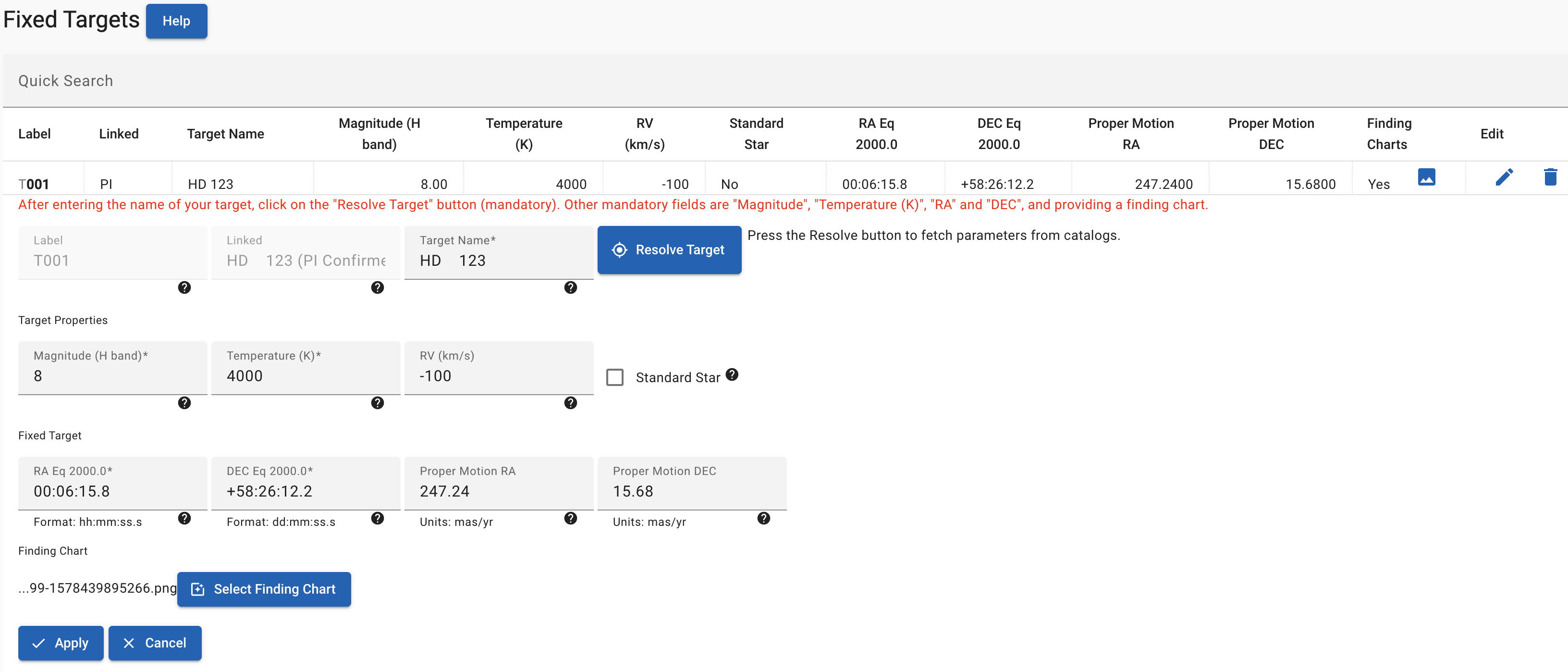
| Target name | After entering the name of a
target, please use the "Resolve target" button. Values retrieved from
CDS will be displayed in a popup window. If they are correct, you may
use the "Link Target" selection in that popup window and continue
entering additional values (such as the Temperature). The target will
be indicated as being "PI linked" or "PI Confirmed". Please do not modify the name suggested by CDS; by using proper catalog names, the Data Reduction Software (DRS) will be able to properly associate observations of the same target.
If the target was not resolved by CDS, you may manually enter the
necessary values by using "Custom Target". In this case, the target will
be listed as "Custom Target" or have a Linked value of "No" (not linked
to catalog values). If a target is indicated as being "System Linked",
please use the Resolve Target button to link it to catalog values. |
| Finding chart | Finding charts are mandatory and you are asked to add a finding chart after creating your target. Click on the button "Select Finding Chart" to automatically generate a finding chart with the proper orientation and scale (4 arcmin on a side). You may slide the chart so the cross is centered on your target, but please do not zoom in or out. If the chart generated is unclear or otherwise not useful, you may upload your own chart by clicking on "Select file", as long as its FOV is about 4 arcmin, the
image is in H band, the file is a JPG and a crosshair clearly indicates your target. You may also edit the comment that is
automatically generated (for a binary star, to specify the component to observe for example). |
| Magnitude & Temperature | Provide the estimated/measured magnitude in the H band and the estimated effective temperature. This is to double check S/N calculations. Provide a comment in the Summary if your stars are highly variable and/or this information is not reliable. |
| Position & Proper Motion | Equinox 2000.0 is assumed; coordinate format is expected in the form hh:mm:ss.s and dd:mm:ss.s. Provide a proper motion if it is greater than 50 mas/y. |
| RV | Systemic radial velocity of the star in km/s. This may be useful to confirm the identification of the star, and also helpfull for the data redcution software. |
| Standard star? | This flag must be set when the star is a "standard" star, for instance to be observed multiple times, each time other science targets are observed. Note that hot stars for telluric absorption measurements and RV reference stars are anyway observed every night, under Q58 and Q57 programs. Those Qxx data are publicly available, raw and reduced products are avaible at CADC. Provide your
standard-star observing pattern in the comment section of the summary page. |
| Moving Targets | Moving targets are now supported (22A onward). You have to provide ephemerides following the XML format given in the example file you can download from K2 by clicking on the 'View ephemerides' clock. At least 6 distinct dates must be provided, with the earliest dates possibly 1 or more nights before your night(s) of interest (this to allow us to do telescope pointing verifications if needed). No need to provide constant time sampling. Most important is that ephemerides MUST be topocentric (NOT geocentric) AND astrometric (NOT apparent). Use observatory code T14 to generate topocentric ephemerides suitable for CFHT. We recommand using the JPL Horizons web app to generate your ephemerides. |
| Observing Template |
|---|
|  |
|---|
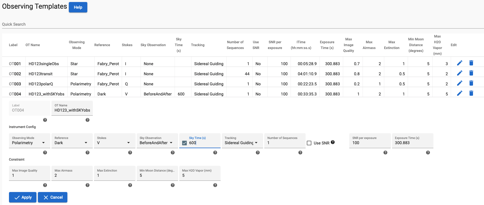
| OT name | Spaces and special characters are possible but not recommended. Names are limited to 68 characters. You don't have to set a label, it is set by the system automatically. |
| Observing Mode | Choose between Spectroscopy ("Star") and "Polarimetry". Choosing Polarimetry will automatically set 4 exposures, each of the requested exposure time. |
| Reference | Choose "Dark" or "Fabry-Perot". Use Fabry-Perot for high-precision radial velocity. Use Dark if your star is fainter than H~11. |
| Stokes | Select "I" if you are using the Star mode. Select your Stokes parameter for Polarimetry. This will set the correct sequence of configurations. In a Polarimetric sequence, 4 exposures are taken. |
| Sky observation | One or two sky observations of 10 min are taken during a SPIRou run for calibration purposes. Telluric corrections are available in the reduced spectra using regularly observed telluric stars and a PCA approach to match your observing conditions. So it is generally not useful to take a sky before or after your targets. Leave this field to "None" if you don't need sky background observations taken spatially and temporally close to your observation. If you do need it (faint stars, persistence to be subtracted, critical K-band observations), select when you want the sky observed: "Before" the target exposure, "After", or "Before and After". By default, a sky exposure will have the same exposure time than the science single exposure. By checking the box 'Sky Time (s)' you can specify the sky exposure time if you want it to be different. |
| Desired SNR | This is the SNR per 2.28 km/s pixel at 1.7 micron. For polarimetric sequences, it is the SNR per exposure (enter 50 if you want to reach 100 after the 4 exposures from one polar sequence). This SNR goal is important as the observer uses it to grade and validate your observation. The observations will be validated if the measured SNR is greater than 70% of the goal. Saturation is reached for SNR>900 at 1.7 micron. |
| Exposure time | This is the requested exposure time in seconds of a single exposure in Polarimetry mode. Max exposure time is 1800s, min is 11s. In SNR mode, the actual exposure time may be shorter than the requested exposure time if observing conditions are very good. Please note that the observatory charges 35s for overheads of each exposure in polarimetric mode and 28s in 'star' mode, so take this into account when comparing to your allocated time. |
| Tracking | We offer two modes of tracking: the standard sidereal mode that compensates for the Earth rotation and the non-sidereal mode to follow moving targets such as Solar System objects, based on the ephemerides you provide (see above Moving Targets section). |
| Number of sequences (consecutive observations in a night) | Enter 1 if you plan to monitor a star with one visit per observing night. In Star mode, sequence and exposure are the same, so enter the number of exposures. If you want to observe a transit, you will increase the number of sequences to the number of exposures you want during the transit: In the example above, we set the number of sequences to 44, to have 44 exposures during the transit, here lasting 4 hours. Note that the number of sequences is not the number of iterations (or visits) on your target during a run or a semester that you will find under the monitor type in the observing group. Note also that in Polarimetric mode, a sequence is composed of 4 exposures: Be carefull to enter the exposure time for one exposure and the number of sequences, not the number of exposures. |
| Use SNR | Check this box if you want your program to be observed at a fixed SNR. This will trigger the exposure to stop when the SNR goal is achieved, or at the maximum exposure time, whatever comes first. |
| Max Image Quality | Enter here the maximum seeing that can be used for your observation in arcsec. Median image quality is 0.65 arcsec. |
| Max Airmass | Enter here the maximum airmass where your observation must be conducted. It is not recommended to observe beyond 2.0 for high precision Radial Velocity, or beyond 2.5 in general. The ADC (atmospheric dispersion corrector) does not correct dispersion beyond airmass=2.5. |
| Max Extinction | Enter here the maximum extinction in the H band that your observation can handle (in magnitudes). |
| Max H2O vapor | This is the maximum H2O column density in mm. The median is 2.5mm for Maunakea. This parameter is being evaluated at the moment of the observation. |
| Observing Group |
|---|
|  |
|---|
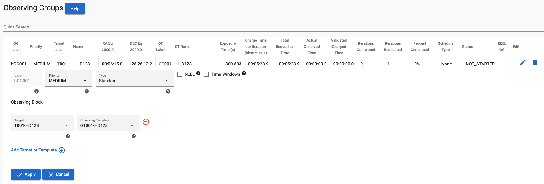
| Observing Group | An Observing Group (OG) connects a Target and an Observing Template (OT) together. If you are concerned by RV precision, use the SPIRou ETC to verify that the expected SNR is in agreement with the RV precision assessed by the ETC based on Figuiera et al 2016 work (chose 'Detailed Output' for the ETC and check the values of RV printed out below the main output table).
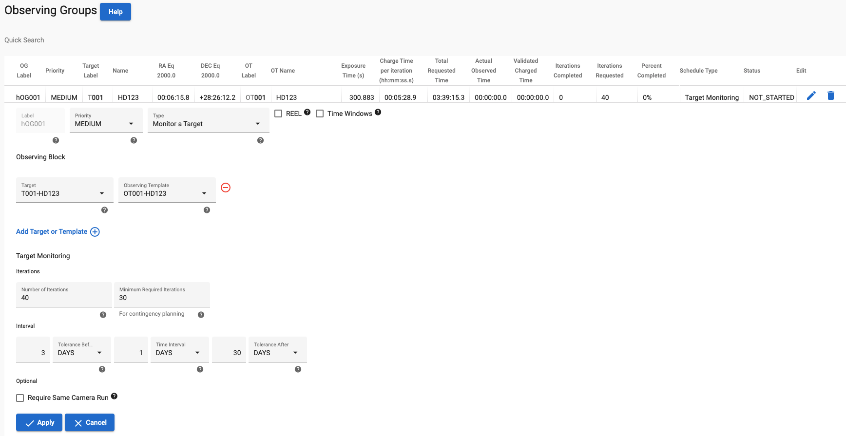
The simplest OG are of the Type "Standard" (shown above) and are used to observe a target once without any time constraint. Targets that need to be observed more than once, with a
regular period, are of the Type "Monitor a Target" (shown below). You have to specify time intervals: 'Tolerance Before' is the time you accept observations to be done in advance of the period you set in 'Time Interval', and 'Tolerance After' is the time you accept the monitoring to be continued after a break in the series. In the example shown, we may start the monitoring even if it's going to introduce a gap of 3 days in the time series, and we will continue the observations only if it will introduce a gap smaller than 30 days with the latest observation done. You can set 'Tolerance after' to 182 days if you want us to observe your target until the end of the semester, whatever the gaps are in the monitoring once it is started. We stop when the number of requested iterations or the allocated time is reached.
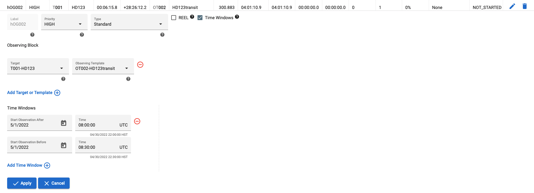
To observe a target only during specific time windows, click the checkbox "Time Windows" and enter as many windows as needed for that OG. You will use this mode to observe transits for example. Note that the time to enter is when your observation needs to be started, independently from OG length itself. The second screenshot below shows a transit observation that has to be started between 8:00 and 8:30 UT. Be carefull time is required in UT. It is also displayed in HST, Hawaii local time, so you can easily verify it's nighttime at CFHT for your observation.
If 2 (or more) OG need to be observed sequentially, with a specific delay between 2 OG, check the box "REEL". REEL connects 2 OG together. In the third screenshot below, selected OG8 is requested to be observed 5 days after OG7.
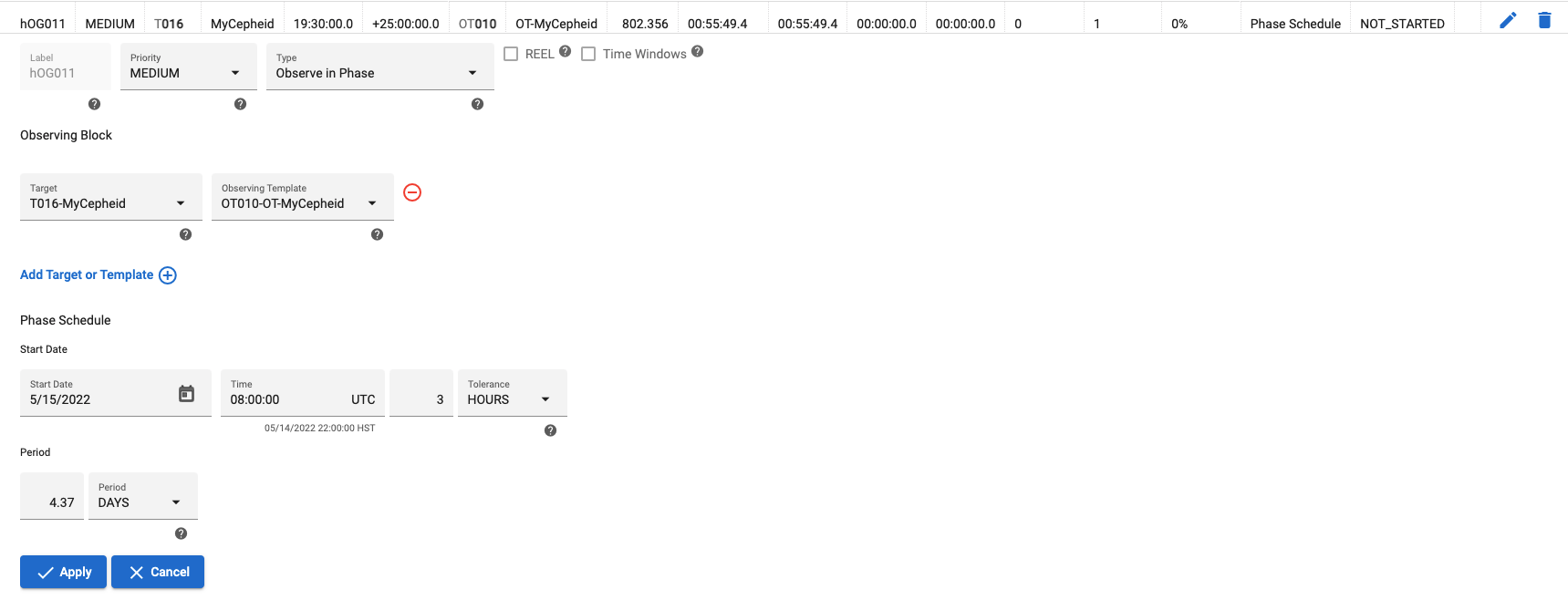
The type "Observe in Phase" is convenient if you have a periodic list of possible dates/times. The OG will only be observed once, on one of the allowed dates/times (last example below).
|
|  |
|---|
|  |
|---|
|  |
|---|
|  |
|---|
| Priority | Indicate your science priority: High, Medium, or Low. It helps the observing team optimizing your program. |
| Link a target and a template | By selecting a target from your list, and an observing template, or several of each, you build up a continuous sequence. An OG can contain several targets and several templates per target, if absolutely required by the observing strategy, for example if a science target must be observed with a standard star. However, keeping it simple (with only one target per OG) and short is the preferred way, as it will insure flexibility and completeness. |
| Additional features |
|---|
| 'Exposures' section | You will note at the very bottom of the page a new section "Exposures". This is where you can follow the progress of your program during the semester. The button "Distribution" will bring you to the data repository for your program. Data reduced at night ("Quicklook") are currently only useful as a first glance and are not recommended for final data analysis. Once a run has ended, all the observations are reduced with the best calibrations possible, and a separate email is sent to the PI to inform them that their data are available. Data are also transferred at CADC but there may be a delay of a few days before they arrive there. |
| Editing | Automatic completion, search filters |
| TBD | |

