|
|
|
MegaCam Raw Data Description
|
Table of contents:
1. Raw data
1.1 Raw data from the camera
The MegaCam focal plane is composed of 40 CCDs E2V CCD42-90 but only the central
36 CCDs are read out as the four CCDs composing the "ears" of the mosaic are almost
fully vignetted by the filter frame (the purpose of the ears is to house the spare
CCDs actually). Hence, the readout image is composed of four stripes of 9 CCDs each.
Each CCD has a 2048x4612 pixels imaging area split into two 1024x4612 imaging areas
as both chip's amplifiers are used. 32 overscan pixels are read out both on the X and
Y axis for both of these amplifiers.
A total of 72 readouts made of 1056x4644 (1024+32 x 4612+32) pixels are saved into a single
Multi-Extension FITS (MEF) file including a primary header describing the structure of the
whole file.
1.2 Raw data format after splicing (archived data)
The camera readout format is however not the most optimal choice for data processing,
hence CFHT decided to archive and process the data into a per CCD reorganized format.
The two amplifier readouts from a single CCD are spliced together into a single file,
with the central rows of the CCDs stiched back together while the overscan region
on the X axis for the first amplifier are pulled to the first rows. It is only
a geometric change, the data remain unchanged in that process.
Figure 1. shows how the data splicing affects the original raw data.
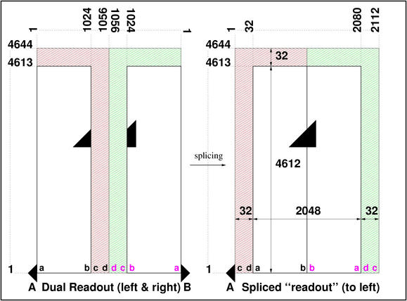
Figure 1. MegaCam FITS splicing data magagement.
The final MEF file is composed of a primary header and 36 extensions going by
the name of "ccdXX", with XX ranging from 00 to 35. Each CCD image has now
2112x4644 pixels with the imaging area found at [33:2080, 1:4612]. Figure 2.
describes the final organization of the data in the mosaic as seen by the
end user (post observation phase). As a general note, notice that the upper
half of the mosaic is flipped 180 degrees in regard to the lower half.
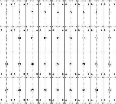
Figure 2. MegaCam readout layout. North is at the top, East to
the left.
New keywords following FITS standards had to be implemented to represent this
way of presenting a multi-readout scheme in a multi-detector file.
- Primary header
The number of extensions keyword is set to 36 and the following block
on HISTORY and COMMENT lines is added to document the new format:
 	HISTORY imsplice: FLIPS ver 2.1 - Elixir by CFHT - Sat Nov 1 2003 -  7:18:26
 	HISTORY imsplice: Splicing the two readouts (A&B) per CCD into a unique image
 	HISTORY imsplice: Splicing results in all detectors as if read from A amplifier
 	HISTORY imsplice: NEXTEND keyword updated (/2) = number of CCDs vs. amplifiers
 	HISTORY imsplice: EXTNAME keyword becomes `ccdxx` instead of `ampxx`
 	HISTORY imsplice: AMPNAME keyword now covers both amplifiers (eg `29a + 29b')
 	HISTORY imsplice: keyword {GAIN, RDNOISE, MAXLIN} replaced by two keywords [A,B]
 	HISTORY imsplice: DATASEC and DETSEC keywords now reflect the entire CCD
 	HISTORY imsplice: BIASSEC becomes irrelevant -> replaced by BSECA & BSECB
 	HISTORY imsplice: New keywords are DETSECA, DETSECB, DSECA, DSECB, TSECA, TSECB
 	HISTORY imsplice: New keywords are ASECA, ASECB, CSECA, CSECB
 	COMMENT Unique detector IDs for MegaCam (North on top, East to the left)
 	COMMENT    --------------------------
 	COMMENT    ba ba ba ba ba ba ba ba ba
 	COMMENT    00 01 02 03 04 05 06 07 08
 	COMMENT --------------------------------
 	COMMENT ba ba ba ba ba ba ba ba ba ba ba
 	COMMENT 36 09 10 11 12 13 14 15 16 17 37
 	COMMENT --------------------------------
 	COMMENT 38 18 19 20 21 22 23 24 25 26 39
 	COMMENT ab ab ab ab ab ab ab ab ab ab ab
 	COMMENT --------------------------------
 	COMMENT    27 28 29 30 31 32 33 34 35
 	COMMENT    ab ab ab ab ab ab ab ab ab
 	COMMENT    __________________________
 	COMMENT The two upper rows of CCDs are flipped, a=A amp, b=B amp
A primary header of a spliced file (724936o) can be found here.
- FITS extension
Many keywords need to be updated as stated in the block added in the primary header; that same block
of information is also added to each extension besides the update and addition of keywords. Here is
a complete listing of the differences between the headers of an "amplifier" extension (before splicing)
and a "ccd" extension (after splicing); a "---" marks the separation before and after the splicing.
The example is taken from ccd13 which is made of amplifiers 26 and 27 (the difference in keywords here
is given for ccd13 vs. amp27).
 	==================================================================================
         < NAXIS1  =                 1056 / Number of pixel columns
 	---
         > NAXIS1  =                 2112 / Number of pixel columns
 	==================================================================================
         < EXTNAME = 'amp27   '           / Extension name
         < EXTVER  =                   27 / Extension version
 	---
         > EXTNAME = 'ccd13   '           / CCD number in the mosaic
         > EXTVER  =                   13 / Now matches the CCD number in the mosaic
 	==================================================================================
         < AMPNAME = '13a     '           / Amplifier name
 	---
         > AMPNAME = '13a + 13b'          / List of amplifiers names for this image
         > AMPLIST = 'A B     '           / List of amplifiers for this CCD
 	==================================================================================
         < DETSEC  = '[12628:11605,14320:9709]' / Mosaic area of the detector
         < DATASEC = '[1:1024,1:4612]'    / Imaging area of the detector
         < BIASSEC = '[1025:1056,1:4644]' / Overscan area of frame
 	---
         > DETSEC  = '[12628:10581,14320:9709]' / Mosaic area of the entire readout
         > DETSECA = '[12628:11605,14320:9709]' / Mosaic area of the A readout
         > DETSECB = '[10581:11604,14320:9709]' / Mosaic area of the B readout
         > DATASEC = '[33:2080,1:4612]'   / Imaging area of the entire CCD in raw frame
         > BIASSEC = '[0:0,0:0]'          / Dual amplifiers readout - see BSECA & BSECB
         > ASECA   = '[1:1056,1:4612]'    / Section by A amplifier in raw frame
         > DSECA   = '[33:1056,1:4612]'   / Image area of A amplifier in raw frame
         > TSECA   = '[33:1056,1:4612]'   / Trim section of A amplifier = DSECA
         > BSECA   = '[1:32,1:4644]'      / Overscan of A amplifier in raw frame
         > CSECA   = '[1:1024,1:4612]'    / Section in full CCD after BSECA cut out
         > ASECB   = '[1057:2112,1:4612]' / Section by B amplifier in raw frame
         > DSECB   = '[1057:2080,1:4612]' / Image area of B amplifier in raw frame
         > TSECB   = '[1057:2080,1:4612]' / Trim section of B amplifier = DSECB
         > BSECB   = '[2081:2112,1:4644]' / Overscan of B amplifier in raw frame
         > CSECB   = '[1025:2048,1:4612]' / Section in full CCD after BSECB cut out
 	==================================================================================
         < MAXLIN  =                65535 / Maximum linearity value (ADU)
 	---
         > MAXLIN  =                65535 / Level at 1% linearity departure (ADU) = Average
         > MAXLINA =                65535 / Level at 1% linearity departure (ADU) A amp
         > MAXLINB =                65535 / Level at 1% linearity departure (ADU) B amp
 	==================================================================================
         < GAIN    =                 1.66 / Amplifier gain (electrons/ADU)
         < RDNOISE =                  3.9 / Read noise (electrons)
 	---
         > GAIN    =               1.6900 / Converting gain (e-/ADU) = Average [A,B] amps
         > GAINA   =               1.6600 / Converting gain of A amplifier (e-/ADU)
         > GAINB   =               1.7200 / Converting gain of B amplifier (e-/ADU)
         > RDNOISE =                    3 / Read noise (electrons) = Average [A,B] amps
         > RDNOISEA=                    3 / Read noise (electrons) A amplifier
         > RDNOISEB=                    4 / Read noise (electrons) B amplifier
 	==================================================================================
The FITS header of a spliced file for ccd13 (724936o) can be found here.
|
2. CCD characteristics per amplifier
The following characteristics were derived from transfer curves obtained with
the LED internal calibration sources at the back of the MegaCam shutter. They
provide a stable and controlled light source allowing the measurement and follow-up
of the camera characteristics over time.
2.1 Noise
The noise was derived from the standard deviation of a 20x20 pixels box. The median
noise over the mosaic (all 72 amplifiers) is 4.2 electrons, with a dispersion of
about 0.6 electrons across the mosaic. The most extreme values are 7.6 electrons
(amplifier A of CCD08), and 3.7 electrons (amplifier A from CCD20).
2.2 Gain
The gain per amplifier was derived from a fit on the transfer curve. The average
gain over the mosaic is 1.67 electrons per ADU with a dispersion of about 0.2. The
most extreme values are 2.06 (amplifier A from CCD17) and 1.51 (amplifier A from CCD20).
2.3 Linearity
The linearity residual over the dynamic of the CCD was derived from a linear fit across
the points. Typical non-linearity is close to 1 percent but a few CCDs have a slightly
higher non linearity:
- CCD12: ~2,2% for both amplifiers
- CCD17: ~1.8% for both amplifiers
- CCD23: ~1.8% for the A amplifier
- CCD33: ~1.7% for both amplifiers
- CCD28: ~1.7% for both amplifiers
- CCD20: ~1.6% for both amplifiers
- CCD13: ~1.6% for both amplifiers
- CCD22: ~1.6% for both amplifiers
2.4 Summary table
A summary table of the amplifiers characteristics derived from the
transfer curve ran in December 2002 can be found here.
|
3. CCD raw data features
3.1 Overscan level
The overscan along the Y axis presents a gradient of up to 10 ADUs. In consequence
this gradient must be properly modeled and subtracted to the frame at the preprocessing
stage. The median level of the overscan also changes slightly over long timescales
(say hours) by as much as 10 ADUs for some amplifiers.
Figure 3 shows a cut along the entire height of CCD13 (the range of the gradient is
5 ADUs).
Figure 3. MegaCam overscan structure along the Y axis.
3.2 Bias structures
After being corrected for the varying overscan, a bias frame does not
exhibit any large 2D scales structures. However two features are present:
- Pixel ringing
A pixel ringing can be seen on the first 30 pixels read in the
imaging area. The amplitude is fairly low, from +5 ADUs to -1 ADU.
This feature is properly corrected on the science frames by subtracting
a bias frame. Figure 4. shows this phenomena which is due to the video
chain "warmup" time at the beginning of a new line (the structure
is uniform over the whole height of the CCD and for each amplifier). Notice
on this Figure 4. that the image is only ~90x70 pixels and the first 32
pixels on the left are from the artificial data stitching due to the
data splicing. The first pixels read from the camera are actually
the bright ones.
Figure 4. MegaCam pixel ringing at the beginning of each line. 90x70 pixels zoom.
Amplitude is +5 ADUs to -1 ADU.
- Noise bands
The MegaCam controller introduces very low level
structures during the readout. The amplitude is within
1 ADU and these structures disapear in the sky background
photon noise even on short exposures.
Figure 5. 1 ADU level horizontal structures introduced
during the readout. Image size is ~500x300 pixels.
3.3 Dark current
The focal plane is kept at a temperature of -130 deg. C., low
enough for basically not getting any dark current generation.
Indeed, the average dark current measured on the images does
not exceed 0.1 electron per pixel per minute, this is less
than 2 ADUs on a 30 minutes exposure.
3.4 Bad pixels
The cosmetic of the MegaCam focal plane is outstanding with
only 0.2% of the pixels having to be masked. Here are the
various types of blemishes found across the focal plane:
- Blocked column:
It is caused by a strong trap that blocks any charge
transfer from pixels further up on the same raw.
A few dozens across the whole mosaic.
- Hot column:
It is caused by a very hot pixel injecting charges
in the electrons clouds from pixels further up on the
same raw as they pass over the hot spot during the
transfer. A couple across the whole mosaic.
- Quantum efficiency "dip" / bad pixels cluster:
It is caused by a strong local decrease in quantum
efficiency. It can be so strong for some of them
that the flat-fielding will sort of work but the
noise in that area will be much higher. This is
the most commonly found blemish on MegaCam raw data.

Figure 6. A bad column (left) and a cluster of bad pixels (right).
3.5 Flat-fields in broadband filters
The twilight flat-fields for use in MegaCam data processing
are taken when the sky is still dominated by the Rayleigh scattering
(vs. the OH airglow) to avoid in particular having any fringes
in the i' and z' bands.
For the u* and g' band, the main visible features are the
'cross-hatch' diamond patterns resulting from the laser annealing
process after thinning of the CCD wafer.
In the i' and z' band, large scale structures are also associated
to the thinning process as regions of the chip are on an average
thinner than others, resulting in a lesser efficiency at interacting
with near infrared photons.
Figure 7. Single CCD twilight flat-fields in the u*, g', r', i' and z'
broadband filters.
3.6 Fringes
Fringes are systematically present of i' and z' band images and
at the level of respectively 6% and 15%. They can occasionally
be seen on r' band images at the level of 0.5%.

Figure 8. Fringes in the i' band: full CCD (left) and region (right).
3.7 Cosmic rays
The rate of cosmic rays hits is standard with approximately
150 events per CCD per minute. Due to the extreme thinness
of the CCDs (16 microns), most events occupy only a few
adjacent pixels. In broadband filters observations, most
of them get "erased" in the sky photon noise.

Figure 8. Typical cosmic rays hits recorded on a long dark exposure.
|
4. Mosaic raw data features
4.1 Quantum efficiency & gain
Since quantum efficiency varies from CCD to CCD, and so does the gain
from amplifier to amplifier, a raw image with flux on it (a science
frame or a flat-field) will show a clear signature of the mosaic.
Figure 9. A raw mosaic flat-field in the u* (left) and i' (right) bands.
4.2 Central "dip" in the g' band
The g' band image exhibit a sensitivity dip due to the optics at
the center of the field at a 5% level but it gets perfectly corrected
by the flat-fielding process.
Figure 10. A raw mosaic flat-field in the g' band.
|
|
|